Project Planning
An Overview and Example of Using Monte Carlo Analysis in Project Planning
Risk in Project Planning
In this article we will discuss how to model risk in project planning. Two primary sources of risk are time and cost; we'll focus on time because it is slightly more complicated; a similar analysis can be applied to cost planning (See note 1).
The risk in planning for project completion time is, naturally, that your projections are incorrect. Underestimating project time can result in additional costs and potential penalties. Overestimating project time can result in wasted resources.
With practice, and good analytical techniques, you can generally construct a reasonable projection for project completion time. But in the real world, it's not possible to anticipate every contingency, and even the best project planning will include some over- or underestimates.
To take this reality into account, it's common in project planning to produce multiple estimates for project completion time. Estimating best-case, worst-case, and expected estimates gives you a range of completion times, and tries to take into account the risk of unanticipated factors.
The Basic Project Plan
Consider a simple project plan. This plan includes a single project, with three tasks:
| Task | Best-Case | Expected | Worst-Case |
|---|---|---|---|
| Task 1 | 10 Days | 20 Days | 30 Days |
| Task 2 | 10 Days | 20 Days | 30 Days |
| Task 3 | 5 Days | 10 Days | 20 Days |
Let's further assume that these tasks must be completed in sequence, meaning each task is dependent on the task before it. How long will the project take to complete?
You can look at the projections for each task and add them; this will give you the best-case, expected, and worst-case scenario for the entire project.
| Task | Best-Case | Expected | Worst-Case |
|---|---|---|---|
| Task 1 | 10 Days | 20 Days | 30 Days |
| Task 2 | 10 Days | 20 Days | 30 Days |
| Task 3 | 5 Days | 10 Days | 20 Days |
| Total | 25 Days | 50 Days | 80 Days |
This is useful, but still unrealistic; because it's unlikely that each task will take the best-case time, or the worst-case time. More likely, one task will take a little longer, and another will be completed ahead of schedule.
This is where Monte Carlo analysis can be helpful. Starting with the estimates for the project, we can run an analysis based on random estimates for each task. This will produce a model that takes into account variability, and also considers that each task is independent.
Adding Randomness
To do that, the first step is to add a random variable which models each task. There are two distributions commonly used to do this: the beta-PERT distribution (also called just PERT distribution), and the triangular distribution.
For this example, we will use the PERT distribution. This distribution is used for modelling expert data when, as here, we have estimates for the range of possible values. It takes a minimum, maximum, and most likely value, and returns a sample from that distribution. The distribution creates a smooth curve. For a discussion of the characteristics of the PERT distribution, see this article on our website.
| Task | Best-Case | Expected | Worst-Case | Sample (PERT) |
|---|---|---|---|---|
| Task 1 | 10 Days | 20 Days | 30 Days | 24 Days |
| Task 2 | 10 Days | 20 Days | 30 Days | 16 Days |
| Task 3 | 5 Days | 10 Days | 20 Days | 13 Days |
| Total | 25 Days | 50 Days | 80 Days | 53 Days |
In this case, with random values selected for each task, you can see that the first task takes a little longer than expected. The last task takes longer as well. The second task is completed ahead of schedule.
Overall, this is the sort of thing we would expect to see in the real world; not the best case, not the worst case, but somewhere in between. A single random case is not useful, however, because it represents only one out of essentially limitless possibilities. This is where we can use Monte Carlo simulation to measure understand the risk.
Monte Carlo Analysis
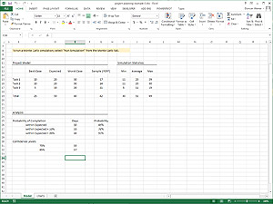
In a Monte Carlo analysis, we run the same model — selecting a random value for each task — but we do it hundreds or thousands of times. Each time it runs, we record the values. When the simulation is complete, we can look at statistics from the simulation' to understand the risk in the model.
We'll start with the basic statistics: the minimum, maximum, and average.
| Task | Best-Case | Expected | Worst-Case | Sample (PERT) | Minimum | Average | Maximum |
|---|---|---|---|---|---|---|---|
| Task 1 | 10 Days | 20 Days | 30 Days | ... | 11 Days | 20 Days | 29 Days |
| Task 2 | 10 Days | 20 Days | 30 Days | ... | 10 Days | 20 Days | 29 Days |
| Task 3 | 5 Days | 10 Days | 20 Days | ... | 5 Days | 11 Days | 19 Days |
| Total | 25 Days | 50 Days | 80 Days | ... | 32 Days | 51 Days | 70 Days |
Three notes about this table before we continue:
This data comes from a Monte Carlo analysis of 1,000 trials.
The last row contains statistics calculated from the total — these are not sums of the columns above them. If this is not clear, please see note 2.
The statistics are rounded to the nearest day. The actual average for the total, for example, was 50.83.
The first thing we can take away from this data is that the average completion time is close to our central estimate. That is what we would expect; it's the most likely case for each task. Next, we can see that the best and worst cases from the simulation — the minimum and maximum of the total — are not as extreme as the absolute best and worst cases, if we just summed up the estimates.
That is to be expected as well, because the tasks are independent. Even if one task takes the worst-case time, it's not necessarily likely that another task will meet the worst-case estimate. The Monte Carlo model helps capture this independent variability, and allows us to tighten up the estimates a bit. We can now say that the worst case scenario is 70 days, instead of 80.
Next, we can look at the range of data generated during the Monte Carlo simulation to understand more about the projections.
Probability Analysis
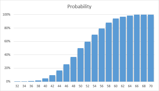
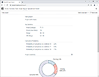
This chart plots the time, in days (at the bottom), against the probability (on the left) of completion within that time. It shows there is only a 5% chance that the project will be completed within 40 days; but there is a 94% chance the project will be completed within 60 days.
What does that mean? When we ran the Monte Carlo simulation, we used random values for each task (based on the estimates), and found the total time for the project. We did that 1,000 times, and each time different random values were selected, resulting in a new random total.
When the simulation was complete, we look at every trial and count the number of times that the total was 40 days or less. We find that in only 5% of the trials (50 out of 1,000) the total project time was 40 days or less. We can therefore say that, during the simulation, there was a 5% probability that the project was completed within 40 days.
Similarly, during the simulation there was a 94% chance that the project was completed within 60 days.
We can also reverse the question, and ask what the completion time was — based on probability from the simulation — at various probability levels. If we want to be 80% sure that the project will be complete, for example, we need to budget 57 days for the project; because in 80% of the cases the project took at least 57 days to complete.
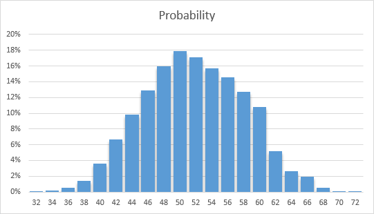
The above chart looks at completion on or before a particular date; in order to prevent under-utilization of resources, we might also consider the actual completion date. We won't address that in this discussion, but the chart looks like this:
Key Points
Based on this analysis, we can find a couple of key points from the model and the analysis:
Estimated Range is 32-70 Days
Even though our best- and worst-case estimates result in totals of 25-80 days, from the simulation we can project that the range will actually be narrower.
Probability of Completion within 50 Days is 50%
Our original estimate was 50 days. The probability of hitting this target, based on the model, is only 50%. That might seem obvious, but it's actually only because this is a very simple model. When you have a more complex model with dependencies between tasks and subprojects, the probability of the "Most Likely" value can often be quite different.
For 75% Confidence, Budget 55 Days; for 85% Confidence, Budget 58 Days
We can say that in 75% of the simulation trials, the project was completed within 55 days. We can budget for various confidence levels by looking at probability from the simulation.
Caveats & Conclusion
The analysis above, and the data taken from the simulation, is entirely based on the project estimates we created in the first step. The validity and the usefulness of the analysis, therefore, is only as good as our ability to estimate.
If the estimates are too broad, or too narrow, or even if the "Most Likely" point is at the wrong place between the values, the analysis may misstate the overall risk.
It's also important not to create estimates that are too broad, and assume you can use the analysis to narrow the probabilities.
The estimates are the most important part of the model. That much, in project planning, is a combination of art and skill. Monte Carlo analysis is just a tool that compliments this. If you can generate viable project estimates, however, Monte Carlo analysis can be invaluable in helping identify and understand risks in your project planning models.
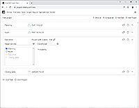
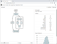
Build a Project Risk Model Online
You can build a project risk model on the web with our new web app. Model projects and tasks, generate project graphs and statistics, and create XLSX files you can run on your desktop.
RiskAMP Project -- Monte Carlo Simulation for Project Planning
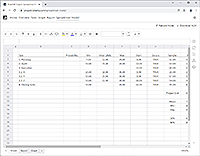
Download Sample Spreadsheets
The example files use the RiskAMP Monte Carlo add-in; if you don’t have the add-in already, you can download a free trial version from our download page.
Download the Example Used in this Article
This file contains the model described in the above note. You can re-run the Monte Carlo simulation, as well as modify various values to see how they impact the analysis.

The first example is relatively simple, for the purposes of describing how the underlying analysis works. This second example contains a more complex model, but it uses an identical analysis.
Notes
We say that time is more complex that cost because tasks can have dependencies, meaning the start of one task might be delayed if another task runs over time. While project cost has its own complexities, accounting for time dependency makes mathematically modelling time projections more difficult.
In this model, because we use a relatively simple project structure, analysis of time and cost is roughly equivalent. In fact you could replace the "days" in the calculation with "dollars" and generate the same analysis.
In the first four columns of the table, the last row is a sum of the values above it. This includes the "PERT" column, where we generate random values for each task. The last row in the PERT column is a sum of the task times.
In the three columns on the right, the simulation statistics, we find the minimum, maximum, and average results for each task. In the bottom row on the right, however, we are not adding the rows above. Rather, we are finding the same statistics — minimum, maximum, and average — for the total value, which was the sum of the PERT column.
We do this because what we are interested in is the combinatorial probability. We want to know what is the minimum value (for instance), when each task is independently randomly selected. As we noted before, sometimes one task will be long and another will be short. In other instances, two tasks will go long. During the simulation we roll the dice, so to speak, and then count up the results. (It's called Monte Carlo simulation after the casino in Monaco).
That's why it's important that we are taking statistics from the total, rather than adding up the statistics from each column. We want to know what is the minimum value when random things happen, as they do in the real world.